Bar chart from pivot table
Remember when you do this you need to refresh the pivot table in background using a simple macro. Of course having a mere pivot calendar is not much fun.

Create A Pivotchart Office Support Chart Pivot Table Sales Report Template
In Excel 2007 and 2010 choose Change Data Source from the Data group of options.

. For instance a bar chart is useful for representing the data under differing conditions such as sales per region while a pie chart can be used to display percentages or portions of a whole. Then we begin to create a stacked column chart from this pivot table. Adjust week start to Monday.
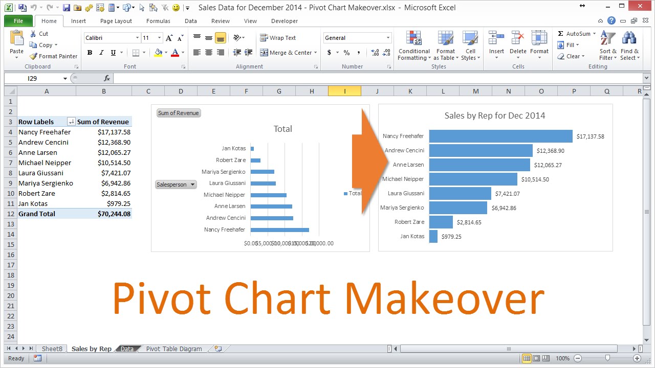
Use this General Section to Change the. On the Y axis we see the company names column 1 in table. Something as shown below.
You will have 2 workbooks open. Next you will want to go to PivotTable Tools - Options on the ribbon Its purple in Office 2010 and click PivotChart. By clicking the Stacked Bar Chart under the Visualization section it automatically converts the Column Chart into Stacked Bar Chart.
Read more Types of Charts in Excel Types Of Charts In Excel Excel offers a variety of chart types based on your requirements. Copy the Worksheet with the Pivot Chart and Pivot Table Twice or more within your workbook. Create and format your Pivot Table and Chart.
Click Change Data Source. Heres how to create a chart from a pivot table step by step so you can take advantage of this useful tool. The bars can be plotted vertically or horizontally.
The Pivot table displays a table of configurable rows and columns with columns showing a count of work. Select the pivot table click Insert Insert Column or Bar Chart or Insert Column Chart or Column Stacked Column. The pie chart groups the 146 active bugs by priority and the bar chart groups the bugs by team and their triage status.
To create a pivot chart from the food sales pivot table follow these steps. Source Data for Pivot Table. How to Create Pivot Chart in Excel.
Click Change Data Source. Locate and launch the Pivot Chart. Kutools for Excels Work Area utility can maximize the working area and hide the whole Ribbon BarFormula BarStatus Bar with just one click.
Format Bar Chart in Power BI General Section. Select your pivot table. First you want to select all data and create a pivot table insert - pivot table Click OK and you will see a blank PivotTable on a new sheet.
How to Format Bar Chart in Power BI. And it also supports one click to restore hidden Ribbon BarFormula BarStatus Bar. Double-click the secondary vertical axis or right-click it and choose Format Axis from the context menu.
You can watch this short video to see the steps for making a pivot table and a clustered stacked column pivot chart. Now the stacked column chart has been created. 1 will replace the original the others are your variations with different data filters etc 2.
I have a pivot table showing 4 columns. In the Create Pivot Chart dialog box make sure you have the range correct and click OK. A Pivot Table is the most powerful feature within Excel as it allows you to analyze your data in many different ways all with a press of a buttonYou can even show the Average in Pivot Table instead of Sum.
Go back to the pivot table tab. Just as you use a Slicer with a Pivot Table you can also use it with Pivot Charts. You can even select 3D Clustered Bar Chart from the list.
Show the selected regions name in the chart title. Next we are adding the English Country Region Name to the Legend section to convert it into the Stacked Bar Chart. I have a pivot graph related to the table.
You can also quickly spot outliers or anomalies in your data. Pivot table could well be the tool that can help us in these crunch situations. Right-click on the Bar representing Year 2014 and select Format.
A bar graph shows comparisons among discrete categoriesOne axis of the chart shows the specific. Click the Next button until you see the screen with the source data range. Next to link the pivot chart to a different pivot table youll move the new pivot chart and set its source data.
Insert a Slicer to the Table. Click Analyze tab Windows or PivotTable Analyze Mac. A vertical line appears in your Excel bar chart and you just need to add a few finishing touches to make it look right.
Notice that several countries had no revenue in Q4 for example. Pivot Chart in Excel. Create a Pivot Chart.
The Summarize Values By option allows you to choose a type of calculation Sum Count Average Max Min Count Numbers Product StdDev StdDevp Var. The last two chart show two different trend views of the active bugs over the last two weeks. There are written steps below the video.
Shop by department purchase cars fashion apparel collectibles sporting goods cameras baby items and everything else on eBay the worlds online marketplace. Add a Pivot table. Delete the original worksheet 3.
The data can be presented based on various categories as it offers a way to apply the pivot table filters that dynamically change the view of the pivot table data. Number of those units with defects 4. A bar chart or bar graph is a chart or graph that presents categorical data with rectangular bars with heights or lengths proportional to the values that they represent.
If you dont select the Pivot Chart before creating the text box the text box will be separate from the chart and therefore wont move along with the Pivot Chart if you ever want to move it With the Pivot Chart selected Go to the Insert tab on the Ribbon. Likewise you can modify your formulas to adjust weekstart to Monday or any other day you fancy. Edit the source data range for your pivot table.
To build a pivot table the data should be in a named Excel table like the one shown below where. A vertical bar chart is sometimes called a column chart. Select the data and go to Insert Charts Pivot Chart.
This will insert a Pivot Chart in a. Youll select the first Bar Chart option and will be greeted by a blank chart. Example pivot table showing revenue per user by country quarter and year.
Rename Worksheets Change Data source filters etc in the table. In the Format Axis pane under Axis Options type 1 in the Maximum bound box so that out vertical line extends all the way to the top. Here is how you can create this dynamic chart.
Original workbook with a pivot table you want to connect the new pivot chart to. Please refer to the Power BI Bar Chart article to understand the steps involved in creating a Power BI Bar chart. Now lets move to the advanced steps of editing this chart.
A pivot table however quickly shows the relationship of this data. This table easily summarizes the data from the previous example. Start by clicking on the bounding border of the Pivot Chart to select it.
Go to the spreadsheet that contains the data for the pivot table 3. Please click on the Format button to see the list of formatting options that are available for this Bar Chart. 2 Link to Different Pivot Table.
Full Feature Free Trial 30-day. Add or change your data. If you want to hide the field buttons right click at any field button to select Hide All.
Using Pivot Calendar as a Chart. Number of units they make 3. Pivot Chart in Excel Table of Contents Pivot Chart in Excel.
One click to hide or show the Ribbon BarFormula BarStatus Bar in Excel. From the Insert Chart dialog box select the All Charts Bar Chart Clustered Bar Chart. Next click in the Formula bar and type an Equal Sign Click on cell G1 which contains the pivot chart title formula.
Most often when the data is big and huge it is difficult to draw conclusions and tell the stories behind the data. Make a Clustered Stacked Column Pivot Chart. S column3column2 The table is ordered form max to min on column 4 that is highest on the top.
In Excel 2003 launch the Wizard utility by right-clicking inside the pivot table and choosing Wizard from the pop-up menu. Create a chart from this pivot table. Next let me add Color to Axis section to create a Bar chart that shows Sales Amount by Color.
This will insert a Simple Clustered Bar Chart. New workbook where the pivot chart was pasted.

Bar Graph Example 2018 Corner Of Chart And Menu Bar Graphs Graphing Diagram

Pin On Chart
Learn How To Create An Interactive Dashboard Using Pivot Tables And Charts In This Video Series Setup Your Source Data An Excel Tutorials Excel Online Student

Learn To Create A Pivot Table And Pivot Chart In Excel Excel Tutorials Pivot Table Intro

Charts In Excel Excel Tutorials Chart Excel

Pivot Tables And Charts In Excel 2010 Excel How To Work With Line Charts 1280 716 Of Best Of Line Graphs Chart Science Graph

Create And Format Charts Using Tableau Desktop 2 Hours Chart Bar Chart Faculty And Staff

How To Compare Values Side By Side Via Bi Directional Bar Charts In Excel Bar Chart Chart Excel

Instead Of Typing Your Pivot Chart Title Use A Worksheet Formula To Create A Dynamic Title Https Www Pivot Table Com 2019 01 09 Get Chart Pivot Table Excel

How To Create A Dynamic Excel Pivot Table Dashboard Chart Excel Dashboard Templates

Excel Pivot Tables Pivot Table Excel Chart

I Will Create Excel Graphs Charts Pivot Tables And Pivot Charts In 2022 Pivot Table Graphing Excel
How To Use Pivot Chart In Excel Pivot Table Excel Excel Tutorials

Excel Dashboard Course 21 Creating A Pivot Table Dashboard With Slicers In Excel In 15 Minutes Youtube Excel Tutorials Pivot Table Excel

How To Use Reports Pivot Tables In Excel In Urdu Advance Excel Pivot Table Excel Free Technology

Multiple Slicer Search Boxes On Dashboards Or Pivot Charts Chart Pivot Table Excel

I Will Make A Good Dashbaord On Excel In 2022 Sales Dashboard Pivot Table Excel